Building Vector Similarity Search in PostgreSQL with pgvector

In this article, you will learn how to implement vector similarity search in PostgreSQL using the pgvector extension, allowing you to find semantically similar results based on meaning rather than keyword matching.

Topics we will cover include:

• What vector embeddings are and how they enable semantic similarity search.
• How to install and configure pgvector, store embeddings in PostgreSQL, and query them using SQL distance operators.
• How to choose the right distance metric and index type for your workload, and how to combine similarity search with standard SQL filters.

Building Vector Similarity Search in PostgreSQL with pgvector

Introduction

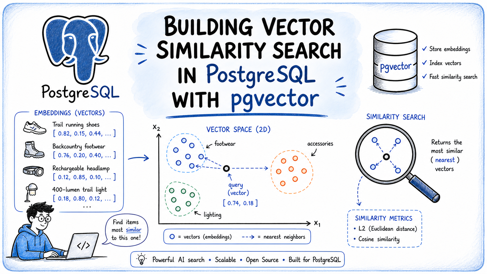
Search works well when users know exactly what they are looking for, but it breaks down when intent is described in natural language. A user searching for “something warm and breathable for high-altitude trekking” will get poor results from a keyword index, because the words in that query rarely align with the words in your data.

This is where similarity search becomes useful. Instead of matching keywords, it finds results based on meaning — connecting user intent to relevant records even when the wording differs entirely.

This article shows how to implement similarity search in PostgreSQL using pgvector. You will learn how to set up the extension, store vector embeddings in your database, and run similarity queries using plain SQL without a separate vector database.

What Is a Vector Embedding?

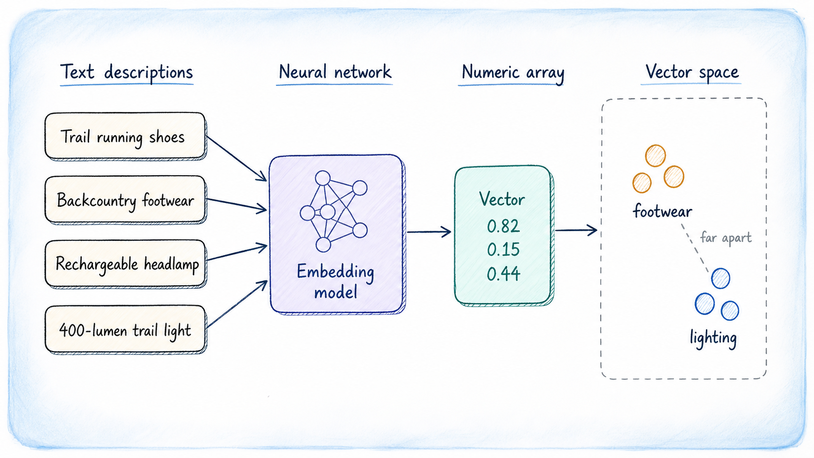
A vector embedding is a list of floating-point numbers that represents the meaning of a piece of data, not its characters or keywords. The numbers are produced by a machine learning model trained to place semantically similar content close together in a high-dimensional numeric space. Two sentences that talk about the same concept will produce embeddings that are numerically close, even if they share no words.

Consider these two phrases:

• “Lightweight trail runners for long-distance hiking”
• “Running shoes built for backcountry endurance”

An embedding model would place their vectors near each other in that space. That proximity is what makes similarity search work: you embed the user’s query, find the stored vectors closest to it, and return those rows.

Generating Embeddings

The vector dimension depends on which model you use. You can choose from several options; the most common ones to try are:

• OpenAI text-embedding-3-small / text-embedding-3-large: 1536 and 3072 dimensions respectively.
• Cohere Embed v4: Multilingual and multimodal, covering text and images in a shared vector space.
• EmbeddingGemma: A 308M parameter open model from Google built on Gemma 3, producing 768-dimensional vectors with Matryoshka truncation support, coverage of 100+ languages, and fully on-device inference.
• BAAI/BGE-M3: Open-source and self-hostable, supporting over 1,000 languages and sequences up to 8,192 tokens. Also available on Hugging Face.
• Sentence Transformers: Lightweight open-source models that run on CPU, suitable for local development where retrieval accuracy is secondary to speed.

The MTEB Leaderboard is a standard reference for comparing embedding models. One rule applies regardless of your choice: the dimension configured in your PostgreSQL column must exactly match the dimension the model produces.

What Is pgvector?

pgvector is an open-source PostgreSQL extension that adds native vector search to your existing database. Rather than moving your embeddings to a dedicated vector store, pgvector keeps them alongside your relational data, preserving PostgreSQL’s transactional guarantees, JOIN semantics, point-in-time recovery, and the full SQL query language.

The extension adds a vector data type for storing embeddings, SQL distance operators for ordering query results by similarity, and two index types — HNSW and IVFFlat — for accelerating nearest-neighbor lookups at scale. It also supports half-precision, binary, and sparse vector types.

Installing pgvector

pgvector supports PostgreSQL 13 and newer. The installation guide in the repository covers every platform in detail; the most common paths are shown below.

On Linux
On Debian and Ubuntu, the APT package is the quickest route. Replace 18 with your PostgreSQL major version:

To compile from source instead, which works on any Linux distribution, use:

On macOS
If you’re on a Mac, Homebrew is the simplest option:

The source compilation steps above work identically on macOS with Xcode Command Line Tools installed.

For Windows, Docker, and conda-forge, see the installation notes in the repository. Once installed, enable the extension in your target database. You only need to do this once per database:

Creating a Table with a Vector Column

We will build a product catalog for an outdoor gear store. Each product has a text description, and we will store an embedding of that description so users can search by meaning.

The vector(1536) column holds one embedding per row. That number must match the output dimension of your model; adjust it accordingly if you use a different one.

For this article we’ll use a smaller test table with 3-dimensional vectors to keep the examples readable:

Inserting Sample Data

In practice you would call an embedding API on each product description at insert time and store the returned vector. Here we use hand-crafted 3-dimensional values that better explain the clustering principle: footwear items share similar first-component values, lighting items cluster around the second, and backpacks share similar third-component values. Embeddings from a model behave the same way.

Running a Query

Now we can search for products similar to a query vector. Imagine a user asks for “trail footwear for rough terrain.” Your application embeds that phrase, and let’s say it receives [0.80, 0.19, 0.40] back from the model. Here is how you find the nearest neighbors:

Output:

The <-> operator computes L2 distance — the straight-line distance between two points in vector space. Lower values mean closer, and therefore more similar. The two footwear items rank at the top, which is what we would expect.

Choosing a Distance Metric

pgvector supports several distance operators, each suited to different data characteristics. Picking the wrong one gives you results that look valid but are subtly incorrect for your use case.

The two distance operators you will use most often are L2 and cosine, and choosing the right one directly affects retrieval quality.

• L2 distance treats vectors as points in space and measures the geometric distance between them. It works best when vector magnitude carries meaningful information.
• Cosine distance is 1 - cosine similarity and measures the angle between vectors rather than their length. This makes it the preferred choice for text embeddings generated by language models.

Most LLM-based embedding APIs produce normalized or near-normalized vectors, where semantic meaning is encoded in direction, not magnitude. Because of this, cosine distance generally delivers more accurate semantic rankings for search and retrieval workloads.

Here is the same query rewritten with cosine distance:

Beyond L2 and cosine distance, pgvector also supports several specialized operators designed for specific use cases:

• Inner product is useful in recommendation systems, where embeddings are trained so that dot products directly represent similarity. Because PostgreSQL only supports ascending index scans on operators, pgvector returns the negative inner product, so you should negate the result to get the actual similarity score.
• L1 distance weights each dimension equally without squaring the differences, giving it mild robustness to outliers compared to L2.
• Hamming and Jaccard apply only to binary vectors, used for memory-efficient quantized representations.

Adding an Index for Performance

Without an index, every similarity query performs a full sequential scan: PostgreSQL computes the distance between the query vector and every row in the table. That is acceptable at ten thousand rows. At a million rows, query latency becomes a serious problem.

pgvector provides two index types for approximate nearest-neighbor search, and each makes a different set of trade-offs.

Hierarchical Navigable Small Worlds (HNSW) constructs a multi-layer graph where each node connects to a bounded number of neighbors across multiple levels of resolution. Queries navigate this graph by entering at the coarsest layer and descending toward the nearest neighbors at increasing granularity. Because the graph is built incrementally, there is no training step, meaning you can create an HNSW index on an empty table and add rows over time without rebuilding. HNSW gives the best speed-to-recall ratio of the two options, but constructing the graph requires more memory and takes longer than IVFFlat.

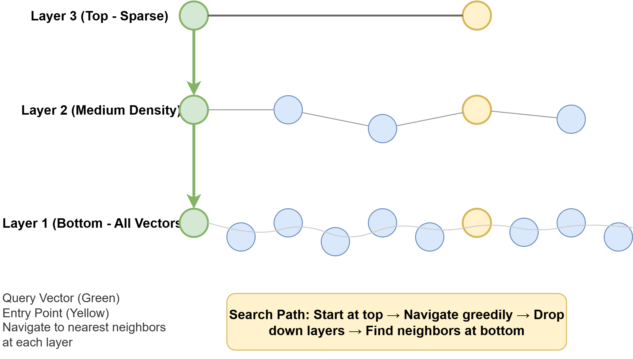
How HNSW Works

Inverted File Flat (IVFFlat) works differently: it partitions the vector space into a fixed number of clusters during index construction, then at query time searches only the clusters closest to the query vector. It builds faster and uses less memory, but those cluster boundaries are fixed at build time. Rows added after construction may land in poorly matched clusters, which can erode recall over time.

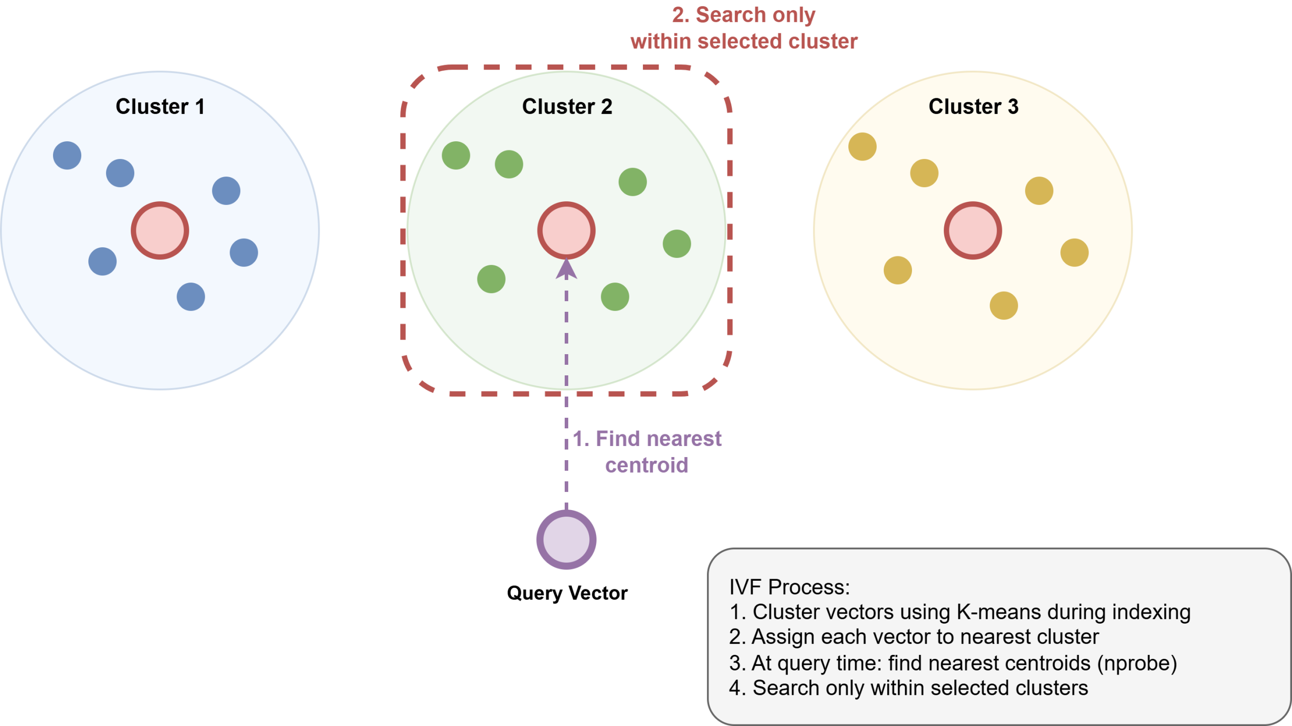
How Inverted File Index Works

Here is how to create an HNSW index for cosine distance:

m sets the maximum connections per node in the graph. ef_construction controls the size of the candidate list during graph construction. Both default to sensible values and only need tuning if recall degrades measurably at scale.

The operator class in your index must match the distance operator in your queries. The mapping is:

If these do not match, PostgreSQL falls back to a sequential scan. Always verify with EXPLAIN that the index is being used when needed.

Putting It Together: Filtered Similarity Search

Similarity search becomes more useful when combined with ordinary SQL filters. pgvector integrates directly with PostgreSQL’s query planner, so you can combine vector ordering with WHERE clauses, JOINs, and aggregations without learning a separate query language.

Here we find the two most similar footwear products to our query, restricting the search to a single category:

Output:

Summary & Next Steps

In practice, most of the complexity comes down to three key decisions:

• Choose your embedding model before writing any schema, because the vector dimension is baked into the column definition and changing it later means re-embedding your entire dataset.
• Match your distance metric to your model’s output. Cosine distance works well for most LLM-generated embeddings.
• Ensure the operator class in your index matches the operator in your queries, because a mismatch produces no error — only a silent regression to full-table scans.

Everything else works exactly as it does in any other PostgreSQL table. The next step is wiring in a real embedding model: call your chosen API on each row’s text at insert time, store the returned vector, and repeat the same call for each user query at runtime. The SQL stays identical to what you have seen here. Happy exploring!