The Machine Learning Practitioner’s Guide to Speculative Decoding

In this article, you will learn how speculative decoding works and how to implement it to reduce large language model inference latency without sacrificing output quality.

Topics we will cover include:

• Why large language model inference is often memory-bound rather than compute-bound.
• How speculative decoding works via draft generation, parallel verification, and rejection sampling.
• How to measure, implement, and apply speculative decoding in real projects.

Let’s get straight to it.

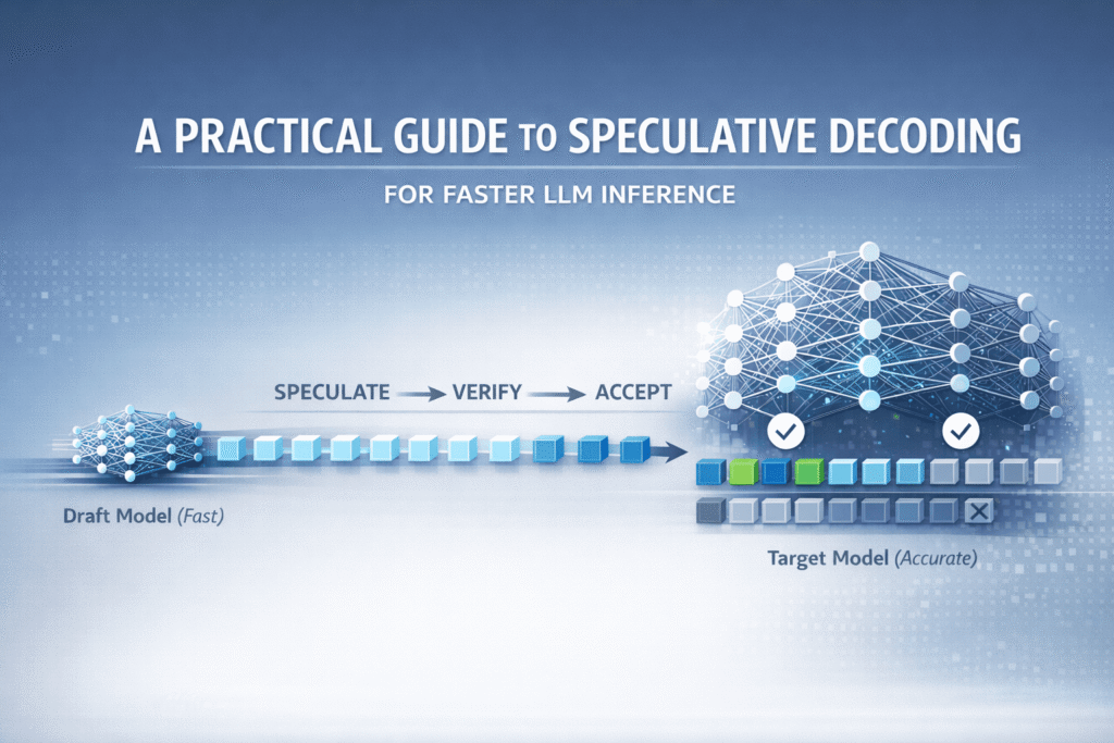
The Machine Learning Practitioner’s Guide to Speculative Decoding
Image by Author

Introduction

Large language models generate text one token at a time. Each token requires a full forward pass through the model, loading billions of parameters from memory. This creates latency in applications and drives up inference costs.

Speculative decoding addresses this by using a small draft model to generate multiple tokens, then verifying them in parallel with a larger target model. The output is similar in quality to standard generation, but you get 2–3× faster inference, and sometimes even more.

Why Large Language Model Inference Is Slow

Before we get into the specifics of speculative decoding, let’s take a closer look at the problem and a couple of concepts that’ll help you understand why speculative decoding works.

The Sequential Generation Problem

Large language models generate text autoregressively — one token at a time — where each new token depends on all previous tokens. The generated token is then appended to the input and fed as the input to the next step.

A token might be a complete word, part of a word, or even a single character depending on the model’s tokenizer.

Here’s what happens during autoregressive generation:

1. The model receives input tokens
2. It runs a forward pass through all its layers
3. It predicts the probability distribution for the next token
4. It samples or selects the most likely token
5. It appends that token to the input
6. Repeat from step 1

For example, to generate the sentence “The scientist discovered a new species” (say, six tokens), the model must perform six complete forward passes sequentially.

The Memory Bandwidth Bottleneck

You might think the bottleneck is computation. After all, these models have billions of parameters. But that’s not quite right because modern GPUs and TPUs have massive computational capacity. However, their memory bandwidth is much more limited.

The problem is that each forward pass requires loading the entire model’s weights from memory into the computation cores. For large models, this can mean loading terabytes of data per generated token. The GPU’s compute cores sit idle while waiting for data to arrive. This is called being memory-bound.

A Note on Tokens

Here’s something interesting: not all tokens are equally difficult to predict. Consider this text:

The scientist discovered a new species in the Amazon. The discovery was made in the Amazon rainforest.

After “The discovery was made in the”, predicting “Amazon” is relatively easier because it appeared earlier in the context. But after “The scientist discovered a new”, predicting “species” requires understanding the semantic context and common research outcomes.

The key observation, therefore, is if some tokens are easy to predict, maybe a smaller, faster model could handle them.

How Speculative Decoding Works

Speculative decoding is inspired by a computer architecture technique called speculative execution, where you perform tasks before knowing if they’re actually needed, then verify and discard them if they’re wrong.

At a high level, the idea is to reduce sequential bottlenecks by separating fast guessing from accurate verification.

• Use a small, fast draft model to guess multiple tokens ahead
• Then use a larger target model to verify all those guesses in parallel in a single forward pass

This shifts generation from strictly one-token-at-a-time to a speculate-then-verify loop. This significantly improves inference speed without a decrease in output quality.

Here are the three essential steps.

Step 1: Token Speculation or Draft Generation

The smaller, faster model — the draft model — generates several candidate tokens, typically three to ten tokens ahead. This model might not be as accurate as your large model, but it’s much faster.

Think of this like a quick-thinking assistant who makes educated guesses about what comes next. As an aside, speculative decoding is also called assisted generation, supported in the Hugging Face Transformers library.

Step 2: Parallel Verification

Okay, we have the tokens from the draft model… what next?

Recall that a single forward pass through the large model produces one token. Here, we only need a single forward pass through the larger target model with the entire sequence of draft tokens as input.

Because of how transformer models work, this single forward pass produces probability distributions for the next token at every position in the sequence. This means we can verify all draft tokens at once.

The computational cost here is approximately the same as a single standard forward pass, but we’re potentially validating multiple tokens.

Step 3: Rejection Sampling

Now we need to decide which draft tokens to accept or reject. This is done through a probabilistic method called rejection sampling that guarantees the output distribution matches what the target model would have produced on its own.

For each draft token position, we compare:

• P(draft): The probability the draft model assigned to its chosen token
• P(target): The probability the target model assigns to that same token

The acceptance logic works like this:

Let’s see this with numbers. Suppose the draft model proposed the sequence “discovered a breakthrough”:

Token 1: “discovered”

• P(draft) = 0.6
• P(target) = 0.8
• Since 0.8 ≥ 0.6 → ACCEPT

Token 2: “a”

• P(draft) = 0.7
• P(target) = 0.75
• Since 0.75 ≥ 0.7 → ACCEPT

Token 3: “breakthrough”

• P(draft) = 0.5
• P(target) = 0.2
• Since 0.2 < 0.5, this token is questionable
• Say we reject it and all following tokens
• The target model generates its own token: “new”

Here, we accepted two draft tokens and generated one new token, giving us three tokens from what was essentially one target model forward pass (plus the draft token generation from the smaller model).

Suppose the draft model generates K tokens. What happens when all K draft tokens are accepted?

When the target model accepts all K draft tokens, the process generates K+1 tokens total in that iteration. The target model verifies the K draft tokens and simultaneously generates one additional token beyond them. For example, if K=5 and all drafts are accepted, you get six tokens from a single target forward pass. This is the best case: K+1 tokens per iteration versus one token in standard generation. The algorithm then repeats with the extended sequence as the new input.

Understanding the Key Performance Metrics

To understand if speculative decoding is working well for your use case, you need to track these metrics.

Acceptance Rate (α)

This is the probability that the target model accepts a draft token. It’s the single most important metric.

\[
\alpha = \frac{\text{Number of accepted tokens}}{\text{Total draft tokens proposed}}.
\]

Example: If you draft five tokens per round and average three acceptances, your α = 0.6.

• High acceptance rate (α ≥ 0.7): Excellent speedup, your draft model is well-matched
• Medium acceptance rate (α = 0.5–0.7): Good speedup, worthwhile to use
• Low acceptance rate (α < 0.5): Poor speedup, consider a different draft model

Speculative Token Count (γ)

This is how many tokens your draft model proposes each round. It’s configurable.

The optimal γ depends on your acceptance rate:

• High α: Use larger γ (7–10 tokens) to maximize speedup
• Low α: Use smaller γ (3–5 tokens) to avoid wasted computation

Acceptance Length (τ)

This is the average number of tokens actually accepted per round. There’s a theoretical formula:

\[
\tau = \frac{1 – \alpha^{\gamma + 1}}{1 – \alpha}.
\]

Real-world benchmarks show that speculative decoding can achieve 2–3× speedup with good acceptance rates (α ≥ 0.6, γ ≥ 5). Tasks that are input-grounded, such as translation or summarization, see higher speedups, while creative tasks benefit less.

Implementing Speculative Decoding

Let’s implement speculative decoding using the Hugging Face Transformers library. We’ll use Google’s Gemma models: the 7B model as our target and the 2B model as our draft. But you can experiment with target and draft model pairings. Just remember that the target model is a larger and better model and the draft model is much smaller.

You can also follow along with this Colab notebook.

Step 1: Installing Dependencies

First, you’ll need the Transformers library from Hugging Face along with PyTorch for model inference.

This installs everything needed to load and run large language models efficiently.

Step 2: Loading the Models

Now let’s load both the target model and the draft model. The key requirement is that both the target and the draft models must use the same tokenizer.

To access gated models like Gemma, you need to log in to Hugging Face.

First, get a Hugging Face API token. Go to huggingface.co/settings/tokens and create a new access token (ensure it has at least “read” permissions).

Option 1 (Recommended in Colab): Run the following code in a new cell and paste your token when prompted:

Option 2 (Environment Variable): Set the HF_TOKEN environment variable before running any code that accesses Hugging Face. For example:

For gated models, you also need to visit the model’s page on Hugging Face and accept the license or terms of use before you can download it. Once authenticated and approved, you can download the model and use it.

Step 3: Preparing Your Input

Let’s create a prompt and tokenize it. The tokenizer converts text into numerical IDs that the model can process.

The tokenizer splits our prompt into tokens, which will serve as the starting context for generation.

Step 4: Implementing Autoregressive Inference (Baseline)

First, let’s establish a baseline by generating text the standard way. This will help us measure the speedup from speculative decoding.

Step 5: Generating With Speculative Decoding

Now let’s enable speculative decoding. The only change is adding the assistant_model and num_assistant_tokens parameters to tell the target model to use the draft model to generate num_assistant_tokens per speculation round.

You should typically see around a 2× improvement. Again, the speedup depends on the target-draft pairing. To sum up, the draft model proposes tokens, and the target model verifies multiple candidates in parallel, significantly reducing the number of sequential forward passes through the larger model.

When to Use Speculative Decoding (And When Not To)

Based on the research and real-world deployments, here’s when speculative decoding works best:

Good Use Cases

• Speculative decoding speeds up input-grounded tasks like translation, summarization, and transcription.
• It works well when performing greedy decoding by always selecting the most likely token.
• It is useful for low-temperature sampling when outputs need to be focused and predictable.
• Useful when the model barely fits in GPU memory.
• It reduces latency in production deployments where adding GPUs is not an option.

When You Don’t Need Speculative Decoding

• Speculative decoding increases memory overhead because both models must be loaded.
• It is less effective for high-temperature sampling such as creative writing.
• Benefits drop if the draft model is poorly matched to the target model.
• Gains are minimal for very small target models that already fit easily in memory.

Let’s wrap up with a note on how to choose a good draft model that offers non-trivial improvement in inference times.

Choosing a Good Draft Model

As you might have guessed, the effectiveness of speculative decoding depends on selecting the right draft model. A poor choice will give you minimal speedup or even slow things down.

The draft model must have:

1. Same tokenizer as the target model. This is non-negotiable.
2. At least 10× fewer parameters than the target. If your draft model is too large, then draft token generation is going to be slow as well, which defeats the purpose.
3. Similar training data to maximize acceptance rate
4. Same architecture family when possible

For domain-specific applications, consider fine-tuning a small model to mimic your target model’s behavior. This can significantly boost acceptance rates. Here’s how you can do that:

1. Collect outputs from your target model on representative inputs
2. Fine-tune a small model to predict those same outputs

This extra effort pays off when you need consistent high performance in production. Read Get 3× Faster LLM Inference with Speculative Decoding Using the Right Draft Model to learn more.

Wrapping Up

Speculative decoding offers a practical way to speed up large language model inference without sacrificing output quality. By using a smaller draft model to propose multiple tokens and verifying them in parallel with the target model, you can achieve 2–3× speedups or more.

The technique works because it addresses the fundamental memory-bound nature of large language model inference, reducing the number of times you need to load the full model’s parameters from memory. While the effectiveness still depends on factors like draft model quality and acceptance rate, speculative decoding is useful in production systems where latency and cost matter. To learn more, check out the following resources:

We’ll cover more inference optimization techniques in the next articles, exploring additional methods to make your large language model applications faster and more cost-effective.